Remote Sensing - Lab 6

Goal and Background:
The goal of this lab was to be introduced to geometric correction, an important preprocessing exercise.  Skills were developed in the two major types of geometric correction often performed on satellite images: spatial and intensity interpolation.  These are normally part of the preprocessing activities used prior to the extraction of biophysical and socioeconomic information from satellite images.  Figure 1 shows


Methods:  
Part 1: Image-to-map rectification
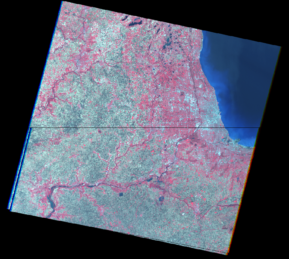
In this part, an image of the city of Chicago was spatially and intensity interpolated using a map as a reference.  Only a first order was used in this interpolation, with a 4 GCP's used.  Nearest neighbor was used in resampling.  Figure 1 shows the GCP's on both the reference map and the original image.  Figure 2 displays the new output image compared with the original image using the swipe tool.

Part 2: Image-to-image rectification
In this part, an image was spatially and intensity interpolated using an image as a reference.  This part used a third ordered interpolation and 12 GCP's in order to rectify the images quite closely.  Bilinear interpolation was used in resampling for this part, which created a smoother image compared to part 1.  Figure 3 shows the GCP's on both the reference image and the original image.  Figure 4 shows the new image compared with the original image using the swipe tool.


Results:  

Figure 1

Figure 2

Figure 3

Figure 4

Sources:
Satellite images are from Earth Resources Observation and Science Center, United States Geological Survey. Digital raster graphic (DRG) is from Illinois Geospatial Data Clearing House.

Remote Sensing - Lab 5

Goal and Background:
Recently LiDAR has become one of the most rapidly expanding areas of remote sensing, and understanding this field is a vital part in becoming a well-rounded analyst.  The goal in this lab was to further basic LiDAR knowledge and practice LiDAR data processing and structure.  Specific skills practiced include: processing and retrieving various surface and terrain models, processing and creating an intensity image and other products from point cloud in LAS file format.

Methods:
Part 1: Point cloud visualization in Erdas Imagine
This part consisted of loading all necessary .las as point cloud in order to access the lidar point cloud tiles.  These were visualized using Erdas Imagine before being brought into ArcMap.

Part 2: Generate a LAS dataset and explore LiDAR point clouds with ArcGIS
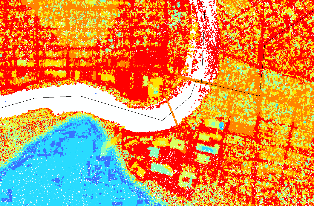
This part consisted of creating an LAS dataset, exploring the properties of LAS datasets, and visualizing it as point cloud in 2D and 3D.  Figure 1 shows the LAS dataset in points by elevation.  Figure 2 shows the walk bridge in the UWEC campus in 2D.  Figure 3 shows the lower UWEC campus in 3D.

Part 3: Generation of LiDAR derivative products
In this part the following derivative products were created:

• Digital Surface Model (DSM) with first return
• Digital Terrain Model (DTM) 
• Hillshade of your DSM
• Hillshade of your DTM

Results:

Figure 1

Figure 2

Figure 3

Figure 4

Figure 5

Figure 6

Figure 7

Sources:
LiDAR point cloud and tile index are from Eau Claire County, 2013.
Eau Claire County Shapefile is from Mastering ArcGIS 6th Edition data by Margaret Price, 2014.

Remote Sensing - Lab 4

Goal and Background:
The purpose of this lab is to continue learning core components of remote sensing while using ERDAS Imagine software to carry out basic remote sensing procedures.

Images often need to be enhanced in ways that make them more easily observable.  It is up to the remote sensing analyst to work with programs and use the procedures available to best enhance these images for the given goal.

Skills obtained throughout the lab include: image subsetting, image fusion, radiometric enhancement techniques, linking image viewer to Google Earth, resampling, image mosaicing, and binary change detection (image differencing) .


Methods: 
Part 1: Image subsetting (creation of area of interest AOI) of study area
This section included creating an inquire box for an image subset, which is shown in Figure 1.  Because the area of interest is often not a perfect rectangle, a second method must be used for an image subset.  Figure 2 shows how shapefiles for Chippewa and Eau Claire counties were used as the area of interest.

Part 2: Image fusion
In this section an image with coarse resolution was combined with a panchromatic image to create a reflective image with a higher spatial resolution.  Using Pan Sharpen, the two images were merged with nearest neighbor as the resampling technique and multiplicative as the algorithm.  When comparing the image with coarser resolution to the new image, the new image was slightly more detailed with evidently smoother features when zoomed in.

Part 3: Simple radiometric enhancement techniques
In this section the haze reduction tool was used to enhance the spectral and radiometric resolution of an image.

Part 4: Linking image viewer to Google Earth
This section involved linking Erdas Imagine images with Google Earth.  This can be helpful because Google Earth has some high resolution images of areas and can serve as a selective interpretation key in remote sensing.

Part 5: Resampling
In this section an image was resampled up in order to decrease pixel size.  When comparing a resampled image to the original image, the new image was smoother and looked less pixelated when zoomed in.

Part 6: Image Mosaicking
This section involved combining two overlapping images together.  This of commonly done when the area of interest lies in both images, so image mosaicking is often necessary.  This process was done twice: once with Mosaic Express (Figure 3) and once with Mosaic Pro (Figure 4).  Each has its strengths and weaknesses, and that can be seen in the results of this lab.

Part 7: Binary change detection (image differencing)
In this section image differencing for two images of the same area taken several years apart.  This showed the changes that occurred from 1991 to 2011.  Once the areas detected to have a significant change in brightness value were identified, that map was brought into Arcmap to make a map of this change, as seen in Figure 6.  Figure 5 shows the distribution of data in the map.


Results:

Figure 1

Figure 2

Figure 3

Figure 4

Figure 5

Figure 6

Sources:
Satellite images are from Earth Resources Observation and Science Center, United States Geological Survey.
Shapefile is from Mastering ArcGIS 6th edition Dataset by Maribeth Price, McGraw Hill. 2014.